Clustering tutorial

After the integration pipeline, we can run clustering in order to discover the cell-type composition of our dataset in an unsupervised way.

Let’s create a clustering folder where we can run our workflow.

Note: if you are in one of the integration folders, you can go up one directory and set yourself at the same level; we prefer to create the clustering folder inside the integration folder after choosing the integrations with panpipes make merge_integration As usual, customize your project folder structure as works best for you!

mkdir clustering && cd $_

now run panpipes clustering config. Inspect and customize the yml (or use the precompiled yml we provide) In the config file, we specify we want to use the teaseq object we have generated in the integration folder, after running the additional batch correction for wnn. We can link it in the folder or specify the full path to the file. The clustering workflow defines what representation is used for the clustering and the clustering parameters. We simply specify which modalities of the object we want to run clustering on, and at which resolution. We can instruct the workflow to run multiple resolutions and they will all be run in parallel.

clusterspecs:
  rna:
    resolutions:
     - 0.2
     - 0.6
     - 1 
    algorithm: leiden # (louvain or leiden)
  prot:
    resolutions:
     - 0.2
     - 0.6
     - 1 
    algorithm: leiden # (louvain or leiden)
  atac:
    resolutions:
     - 0.2
     - 0.3
    algorithm: leiden # (louvain or leiden)
  multimodal:
    resolutions:
      - 0.5
      - 0.7
    algorithm: leiden

Finally, the workflow runs markers analysis across all combinations of clustering and modalities and resolutions tested, plotting the results and saving marker genes files.

Now run panpipes clustering make full --local

Results

After the workfow has finished, you will find in the outputs:

the clustered h5mu object with all the tested combination of clustering parameters on the .obs of the respective modality ,with the clustering of the multimodal representation, in the outer .obs.
a metadata file with all the modality-specific .obs concatenated
a folder for each modality

inside of these:
- the computed umap coordinates with the specified choice of parameters
- one directory for each combination of clustering parameters

Finally, each of the clustering directories contains plots and txt files for the marker analysis. We run the marker analysis using the clustering results and ANY of the modalities. That means you can discover protein markers for clusters that were calculated on RNA, or on ATAC, and viceversa.

Let’s take a look at the rna folder, we can focus on one resolution folder (algleiden_res0.2 in this example):

rna
├── algleiden_res0.2
│   ├── atac_markers.txt
│   ├── atac_markersatac_signif.txt
│   ├── atac_markersatac_signif.xlsx
│   ├── cellnum_per_cluster.csv
│   ├── cellnum_per_sample_id_per_cluster.csv
│   ├── clusters.txt.gz
│   ├── figures
│   │   ├── dotplot__top_markersatac.png
│   │   ├── dotplot__top_markersprot.png
│   │   ├── dotplot__top_markersrna.png
│   │   ├── heatmap_top_markersatac.png
│   │   ├── heatmap_top_markersprot.png
│   │   ├── heatmap_top_markersrna.png
│   │   ├── matrixplot__top_markersatac.png
│   │   ├── matrixplot__top_markersprot.png
│   │   ├── matrixplot__top_markersrna.png
│   │   ├── stacked_violin__top_markersatac.png
│   │   ├── stacked_violin__top_markersprot.png
│   │   └── stacked_violin__top_markersrna.png
│   ├── prot_markers.txt
│   ├── prot_markersprot_signif.txt
│   ├── prot_markersprot_signif.xlsx
│   ├── rna_markers.txt
│   ├── rna_markersrna_signif.txt
│   └── rna_markersrna_signif.xlsx
[...]
├── all_res_clusters_list.txt.gz
├── figures
│   ├── X_umap_clusters.png
│   ├── X_umap_mindist_0.25_clusters.png
│   ├── X_umap_mindist_0.5_clusters.png
│   └── clustree.png
├── md0.25_umap.txt.gz
└── md0.5_umap.txt.gz

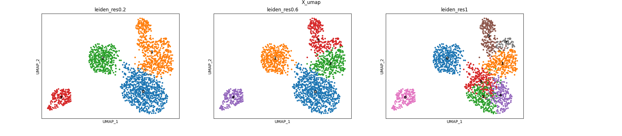
RNA clusters

Here’s what the discovered RNA clusters look like on the computed RNA umap:

for reference, this is what the RNA umap looked like in the integration analysis, using scvi for batch correction:

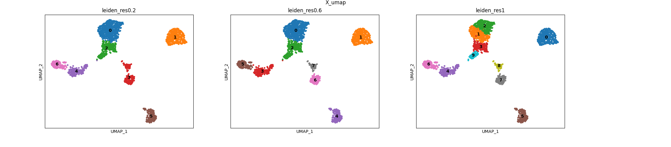
PROT clusters

These are the clustering resolutions we tested on the protein modality:

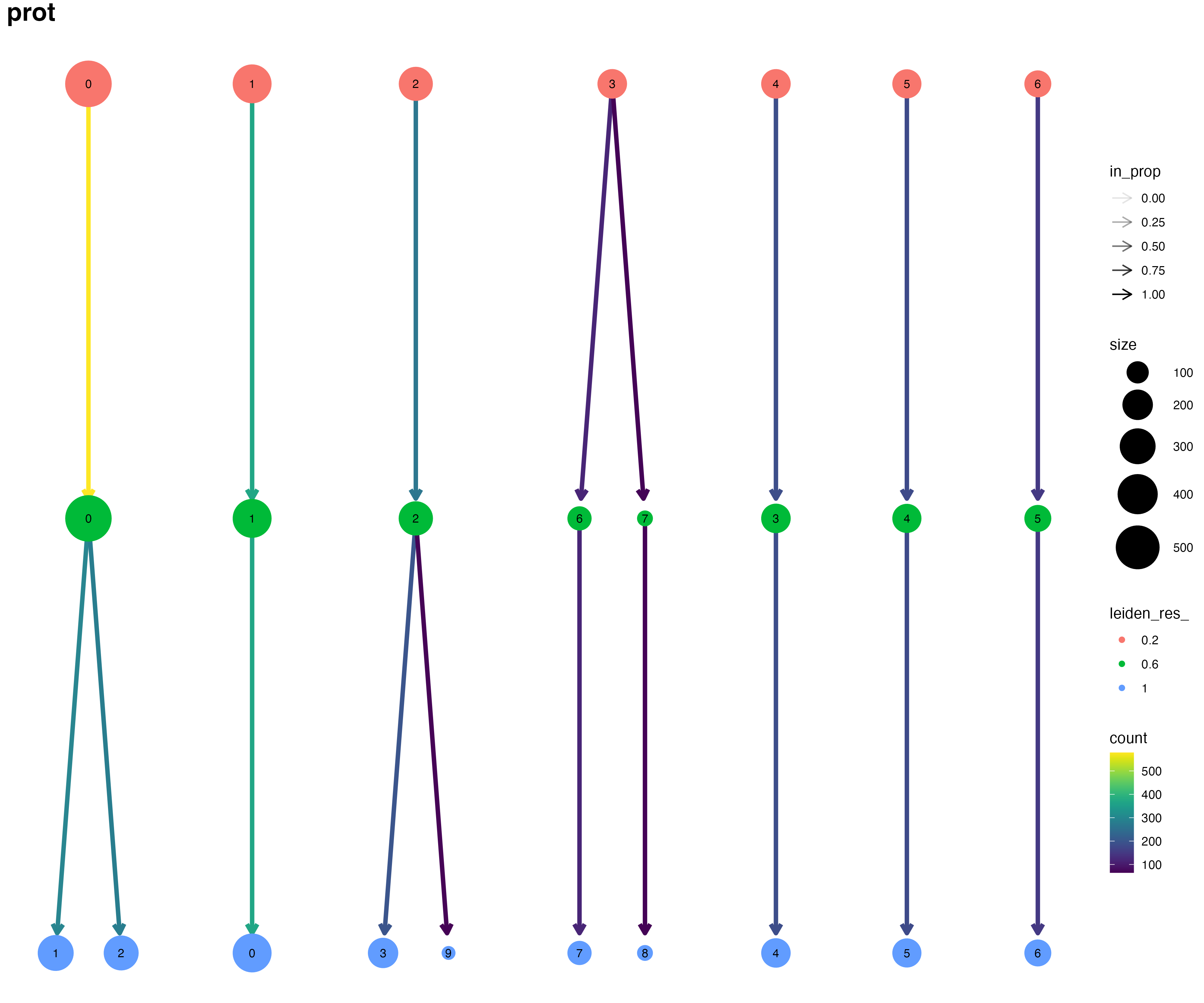
We can use clustree to visualize how the cells are partitioned at increasing resolution parameters. Clustree is ran by default if you request more than one resolution per modality.

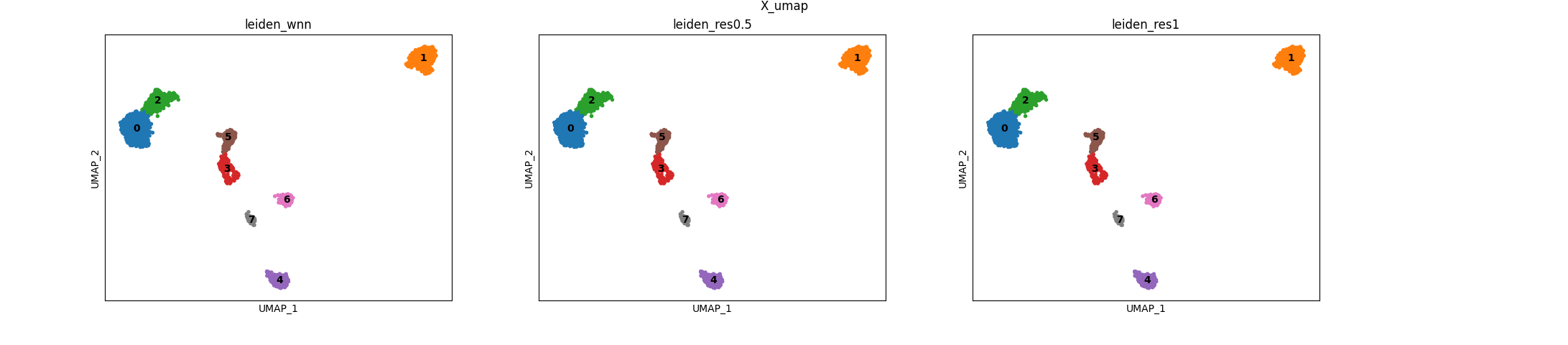
Multimodal clusters

Finally, this is the multimodal clustered representation, we can see that the parameters combination we choose did not yield different clusterings:

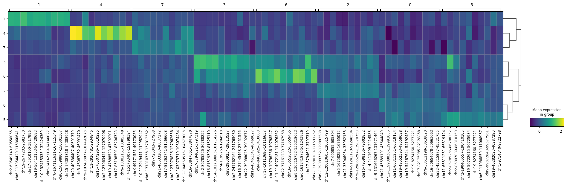
Finally, an example of marker plots, calculated on the multimodal clusters:

RNA markers obtained on multimodal clusters using normalized RNA counts

ATAC markers obtained on multimodal clusters using normalized ATAC counts, summarized by cluster.

For more visualizations, like custom genes expression projected on umaps, please check the visualization tutorial!