Filtering data with panpipes
Running the pipeline
Following the ingest tutorial we now have all the single cell data combined into a single .h5mu object. In the previous tutorial we specified the sample_id: teaseq in the pipeline.yml config file, which ensured we saved the teaseq_unfilt.h5mu object as the main output of the ingest workflow. Within the .h5mu object we stored the computed qc metrics.
It’s time to filter the cells to make sure to exclude bad quality cells for downstream analysis.
In your previously created the teaseq directory, create a new folder to run the panpipes preprocess workflow.
# if you are in teaseq/ingest
# cd ..
mkdir preprocessing && cd preprocessing
In here, run panpipes preprocess config, which will generate again a pipeline.yml file for you to customize. You can review and download the preprocess pipeline.yml here.
Open the yml file to inspect the parameters choice.
If you have run the previous step, Ingesting data with panpipes you will have a *.unfilt.h5mu object that you want to apply filtering on.
This file is the input that we specify in the yaml, where we also specify the modalities that are included in the object:
#-------------------------------
# General project specifications
#-------------------------------
sample_prefix: teaseq
unfiltered_obj: teaseq_unfilt.h5mu

modalities:
  rna:  True
  prot: True
  rep: False
  atac: True
NOTE: it’s important that the .h5mu object is linked (or renamed) in this directory with a sampleprefix_unfilt structure, cause the pipeline will look for this string to start from.
Either copy the file into the directory you have just created or link the file into the new directory (our preferred choice)
cd preprocessing
ln -s ../teaseq_unfilt.h5mu .
# equivalent of
ln -s ../teaseq_unfilt.h5mu teaseq_unfilt.h5mu
If you have a custom .h5mu dataset that you didn’t generate with the panpipes ingest workflow, you can use panpipes preprocess workflow to filter the cells according to your own qc criteria.
In panpipes preprocess workflow, we use a dictionary for filtering, which allows the maximum flexibility to filter your cells and features for each modality, allowing you to provide custom names.
The filtering process in panpipes is sequential as it goes through the filtering dictionary. For each modality, starting with rna, it will first filter on obs and then vars. Each modality has a dictionary in the following format.
# MODALITY
# obs:
  # min:
  # max:
  # bool
# var:
  # min:
  # max:
  # bool
This format can be applied to any modality by editing the filtering dictionary and you are not restricted by the columns given as default.
For example, the filtering in the rna modality retains cells with at least 100 counts and less than 40% mt and 25% doublet scores
#------------------------
# RNA-specific filtering
rna:
    # obs, i.e. cell level filtering
    obs:
      min:
        n_genes_by_counts: 100
      max:
        pct_counts_mt: 40
        pct_counts_rp: 100
        doublet_scores: 0.25
      bool:
Since we’re using the inner join of the mudata object, all the cells passing filtering criteria in all modalities will be retained.
Lastly, in the preprocess workflow we also apply dimensionality reduction (PCA for RNA and PROT, and a choice between PCA and LSI for ATAC )
While it’s common to apply Dimensionality reduction techniques on high-features-numbers assays such as ATAC and RNA, it’s not entirely obvious if it’s beneficial to apply dimensionality reduction on PROT which usually features smaller panels of Features to begin with. This experiment has 47 Features, so we set the number of PCS to 10. If we specify a bigger number of components, the pipeline will automatically reset it to the number of features-1. This is common for all the modalities, although you may never encounter this issue on a big non-targeted RNA experiment!
now run panpipes preprocess make full --local
Look at the log file as it’s generated logs/filtering.log to see what percentage of cells you are filtering based on the selection criteria we specified in the yml.
2023-11-21 18:16:11,864: INFO - Before filtering 2196
2023-11-21 18:16:11,865: INFO - rna
2023-11-21 18:16:11,865: INFO - filter rna pct_counts_mt to less than 40
2023-11-21 18:16:11,883: INFO - Remaining cells 2013
2023-11-21 18:16:11,883: INFO - Remaining cells 2013
2023-11-21 18:16:11,883: INFO - filter rna pct_counts_rp to less than 100
2023-11-21 18:16:11,889: INFO - Remaining cells 2013
2023-11-21 18:16:11,889: INFO - Remaining cells 2013
2023-11-21 18:16:11,889: INFO - filter rna doublet_scores to less than 0.25
2023-11-21 18:16:11,895: INFO - Remaining cells 1917
2023-11-21 18:16:11,895: INFO - Remaining cells 1917
2023-11-21 18:16:11,895: INFO - filter rna n_genes_by_counts to more than 100
2023-11-21 18:16:11,902: INFO - Remaining cells 1914
2023-11-21 18:16:11,902: INFO - filter rna n_cells_by_counts to more than 1
2023-11-21 18:16:11,915: INFO - Remaining cells 1914
2023-11-21 18:16:11,915: INFO - prot
2023-11-21 18:16:11,915: INFO - atac
2023-11-21 18:16:12,229: INFO - intersecting barcodes in rna,prot,atac
2023-11-21 18:16:12,329: INFO - Remaining cells 1914
2023-11-21 18:16:12,329: INFO - (1914, 129082)
2023-11-21 18:16:12,468: INFO - cell_counts
  modality sample_id  n_cells
0      rna    teaseq     1914
1     prot    teaseq     1914
2     atac    teaseq     1914
Let’s take a look at some of the plots produced now.
We can see that we have been effective at filtering some of the cells which lied away from the correlation between the RNA and PROT modalities, looking at the scatterplot of log1p_nUMI in RNA vs PROT across the 3 teaseq samples of the original experiment.

After filtering, we ran normalization, scaling and dimensionality reduction for each modality. We can look at each modality dimensionality reduction, for example the prot PCA highlights a cluster with low UMI counts:

but in the RNA modality, the low-counts cells are distributed across multiple cell groups:
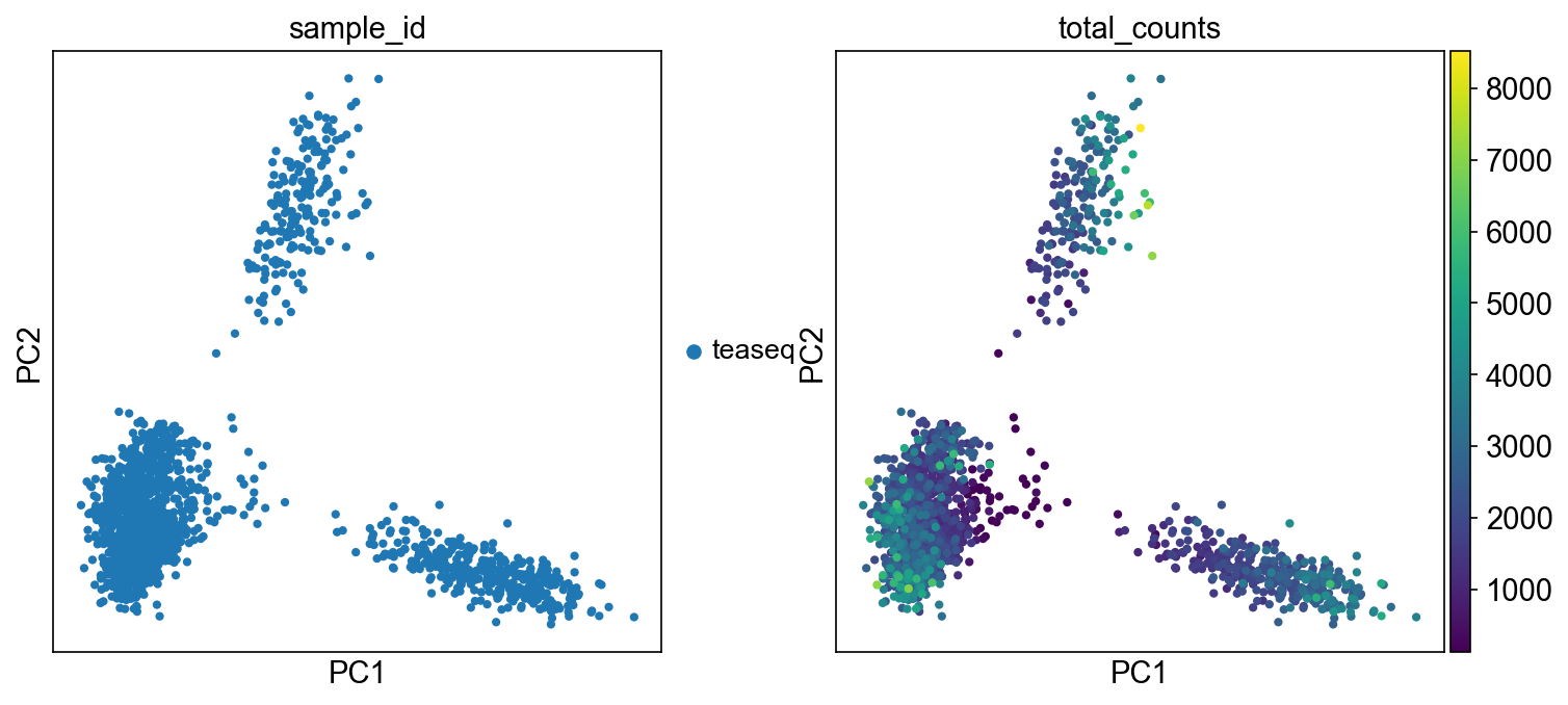
and same for the ATAC:

Changing parameters
You can choose to modify the parameters and re-run a specific task, for example after removing the log file logs/preprocess_rna.log , running panpipes preprocess make rna_preprocess will specifically run the processing task on the rna and exit the pipeline.
If you want to make changes to other parameters like changing normalization methods and then HVG selection and dimensionality reduction, rename the teaseq.h5mu object from the folder and re-run the workflow. (You can also remove all outputs except for the pipeline.yml)
For example, we can change the dimensionality reduction of the ATAC modality from PCA to LSI in the configuration file, as shown in the following excerpt from the pipeline.yml file:
#------------------------------
# ATAC Dimensionality reduction
dimred: LSI  #PCA or LSI
n_comps: 50  #How many components to compute
Then, to apply this change and make sure panpipes re-processes the object with the new dimensionality reduction, we need to remove the previous log file.
Note that we can simply change its name to keep the record of the previous run, i.e. : mv logs/preprocess_atac.log logs/preprocess_log1p_atac.log . The new run will create a new log file logs/preprocess_atac.log reflecting the new request.
We also rename the teaseq object with log-normalized counts and PCA for atac teaseq_atac_pca.h5mu since we will use it later.
Now, to apply these changes, we run panpipes preprocess make full --local again.
After the workflow finishes, we can inspect the resulting MuData and check for changes in the ["atac"] slot. As you can see, we now have a new normalization layer 'signac_norm', a new set of Highly Variable Features and the LSI for the atac modality.
import muon as mu
mdata = mu.read("teaseq.h5mu")
atac = mdata["atac"]
atac
AnnData object with n_obs × n_vars = 1914 × 107739
    obs: 'orig.ident', 'nCount_RNA', 'nFeature_RNA', 'nCount_ATAC', 'nFeature_ATAC', 'original_barcodes', 'n_fragments', 'n_duplicate', 'n_mito', 'n_unique', 'altius_count', 'altius_frac', 'gene_bodies_count', 'gene_bodies_frac', 'peaks_count', 'peaks_frac', 'tss_count', 'tss_frac', 'barcodes', 'cell_name', 'well_id', 'chip_id', 'batch_id', 'pbmc_sample_id', 'DoubletScore', 'DoubletEnrichment', 'TSSEnrichment', 'dataset', 'sample_id', 'n_genes_by_counts', 'total_counts', 'n_counts'
    var: 'features', 'n_cells_by_counts', 'mean_counts', 'pct_dropout_by_counts', 'total_counts', 'highly_variable', 'means', 'dispersions', 'dispersions_norm', 'mean', 'std'
    uns: 'dataset_colors', 'hvg', 'log1p', 'lsi'
    obsm: 'X_lsi'
    varm: 'LSI'
    layers: 'signac_norm', 'raw_counts'

Next uni and multimodal integration
Note: We find that keeping the suggested directory structure (one main directory by project with all the individual steps in separate folders) is useful for project management. You can of course customize your directories as you prefer, and change the paths accordingly in the pipeline.yml config files!