Ingesting 10X Visium data with Panpipes

Let’s run through an example of reading 10X Visium data into MuData objects and computing QC metrics using Panpipes. The workflow describes the steps run by the pipeline in detail.

For all the tutorials, we will append the --local command which ensures that the pipeline runs on the computing node you’re currently on, namely your local machine or an interactive session on a computing node on a cluster.

Create directories and download data

Let’s create a main spatial directory and in that directory, the directories ingestion and data.

mkdir spatial
cd spatial
mkdir ingestion ingestion/data

In this tutorial, we will use two 10X Visium datasets, a Human Lymph node dataset and a Human Heart dataset. To download the two datasets into the data folder, you can use the following commands:

cd ingestion/data 
mkdir V1_Human_Heart V1_Human_Lymph_Node

# download human heart count matrix and spatial info 
cd V1_Human_Heart
curl -O https://cf.10xgenomics.com/samples/spatial-exp/1.0.0/V1_Human_Heart/V1_Human_Heart_filtered_feature_bc_matrix.h5
curl -O https://cf.10xgenomics.com/samples/spatial-exp/1.0.0/V1_Human_Heart/V1_Human_Heart_spatial.tar.gz
tar -xf V1_Human_Heart_spatial.tar.gz

# download human lymph node count matrix and spatial info 
cd ../V1_Human_Lymph_Node
curl -O https://cf.10xgenomics.com/samples/spatial-exp/1.0.0/V1_Human_Lymph_Node/V1_Human_Lymph_Node_filtered_feature_bc_matrix.h5
curl -O https://cf.10xgenomics.com/samples/spatial-exp/1.0.0/V1_Human_Lymph_Node/V1_Human_Lymph_Node_spatial.tar.gz
tar -xf V1_Human_Lymph_Node_spatial.tar.gz

Inside the ingestion directory, you should now have a directory with all the data you downloaded:

data
├── V1_Human_Heart
│   ├── V1_Human_Heart_spatial.tar.gz
│   ├── V1_Human_Heart_filtered_feature_bc_matrix.h5
│   └── spatial
│       ├── aligned_fiducials.jpg
│       ├── detected_tissue_image.jpg
│       ├── scalefactors_json.json
│       ├── tissue_hires_image.png
│       ├── tissue_lowres_image.png
│       └── tissue_positions_list.csv
└── V1_Human_Lymph_Node
    ├── V1_Human_Lymph_Node_spatial.tar.gz
    ├── V1_Human_Lymph_Node_filtered_feature_bc_matrix.h5
    └── spatial
        ├── aligned_fiducials.jpg
        ├── detected_tissue_image.jpg
        ├── scalefactors_json.json
        ├── tissue_hires_image.png
        ├── tissue_lowres_image.png
        └── tissue_positions_list.csv

Please note, that the data folder structure needs to be structured as expected by the squidpy.read.visium function.

Edit submission and yaml file

In spatial/ingestion, create a submission file like the one we provide. For this tutorial, you can use the provided.

In general, the spatial submission file expects the following columns:

sample_id spatial_path spatial_filetype spatial_counts spatial_metadata spatial_transformation

For 10X Visium datasets, only the first four columns need to be specified. With Panpipes you can ingest multiple spatial slides by creating one line for each in the submission file. For each slide, one MuData will be created by the pipeline. Detailed information about the submission file is provided in the usage guidelines

Next, in spatial/ingestion call panpipes qc_spatial config (you potentially need to activate the conda environment with conda activate pipeline_env first!). This will generate a pipeline.log and a pipeline.yml file.

Modify the pipeline.yml or simply replace it with the one we provide. Make sure to specify the correct path to the submission file. If you’re using the provided example yaml file, you potentially need to add the path of the conda environment in the yaml.

Run Panpipes

In spatial/ingestion, run panpipes qc_spatial make full --local to ingest your Visium datasets.

In spatial/ingestion you should now have the following files:

ingestion
├── data
├── figures
│   └── spatial
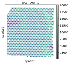
│       ├── spatial_spatial_total_counts.V1_Human_Heart.png
│       ├── spatial_spatial_total_counts.V1_Human_Lymph_Node.png
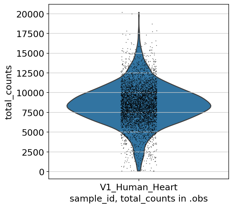
│       ├── violin_obs_total_counts_sample_id.V1_Human_Heart.png
│       ├── violin_obs_total_counts_sample_id.V1_Human_Lymph_Node.png
│       ├── violin_var_total_counts.V1_Human_Heart.png
│       └── violin_var_total_counts.V1_Human_Lymph_Node.png
├── logs
│	├── make_mudatas_V1_Human_Heart.log
│	├── qcplot.V1_Human_Lymph_Node.log
│	├── make_mudatas_V1_Human_Lymph_Node.log
│	├── spatialQC_V1_Human_Heart.log
│	└── qcplot.V1_Human_Heart.log  
├── qc.data # MuDatas with QC metrics 
│	├──	V1_Human_Heart_unfilt.h5mu
│	└──	V1_Human_Lymph_Node_unfilt.h5mu
├── tmp # MuDatas without QC metrics
│	├──	V1_Human_Heart_raw.h5mu 
│	└──	V1_Human_Lymph_Node_raw.h5mu 
├── pipeline.log
├── pipeline.yml
├── sample_file_qc_spatial.txt
├── V1_Human_Heart_cell_metadata.tsv # Metadata, i.e. .obs
└── V1_Human_Lymph_Node_cell_metadata.tsv # Metadata, i.e. .obs

In the qc.data folder, the final MuData objects with computed QC metrics are stored. MuData objects without QC metrics are also available and stored in the tmp folder. The metadata of the final Mudata objects is additionally extracted and saved as tsv files, V1_Human_Heart_cell_metadata.tsv V1_Human_Lymph_Node_cell_metadata.tsv. Using the provided example yaml file, the first rows and columns of the V1_Human_Heart_cell_metadata tsv file should look as follows:

	spatial:in_tissue	spatial:array_row	spatial:array_col	spatial:sample_id	spatial:MarkersNeutro_score	spatial:n_genes_by_counts
AAACAAGTATCTCCCA-1	1	50	102	V1_Human_Heart	0.46748291571753986	1924

With the plots in spatial/ingestion/figures/spatial you can now decide on cutoffs for filtering. The plots include visualizations of the spatial embeddings, as well as violin plots:

Next: filtering and preprocessing using panpipes preprocess_spatial

Note: In this workflow, we have decided to process individual ST sections instead of concatenating them at the beginning, as you saw for cell-suspension datasets. This is because the workflows for processing multiple spatial transcriptomics slides (especially concerning normalization, dimensionality reduction, and batch correction) are still experimental. With panpipes, you can group multiple samples and process them one by one with the same choice of parameters. In the future we will implement the advanced functionalities of SpatialData to deal with multi-sample ST datasets.

Note: We find that keeping the suggested directory structure (one main directory by project with all the individual steps in separate folders) is useful for project management. You can of course customize your directories as you prefer, and change the paths accordingly in the pipeline.yml config files!