Integrating data with panpipes

You have ingested, qc’d and filtered your single cell data and you have now created a .h5mu object with the outputs. It’s time to run integration before applying clustering to discover cell-types in your data.

Go to your previously created teaseq directory and create a new folder to run panpipes integration

# if you are in teaseq/preprocessing
# cd ..
mkdir integration && cd integration

You can now create the pipeline.yml by launching

panpipes integration config

Review and download a preconfigured yml here.

For a description of the algorithms and source references for the methods that will be used below, please check Integration methods implemented in panpipes.

As we did before, we can link the preprocessed h5mu object in the present directory where we will run the integration.

ln -s ../preprocessing/teaseq_atac_pca.h5mu teaseq.h5mu

For this example, we will run some uni and multimodal integration methods. In the yml we specify:

rna:
  tools: harmony,bbknn,scvi
prot:
  tools: harmony,bbknn
atac: 
  tools: harmony,bbknn

and for multimodal integration:

multimodal:
  tools:
    - WNN
    - totalVI
  totalvi:
    modalities: rna,prot
  WNN: 
    modalities: rna,atac,prot 
  mofa: 
    modalities: rna,atac,prot

By default, panpipes will always produce the uncorrected unimodal objects by running neighbours and umap on the baseline dimensionality reduction if present in the object, PCA or LSI depending on the modality. When the dimensionality reduction is not present in the object, panpipes follows the scanpy neighbours default and calculates a PCA with 50 components. If you leave the batch correction arguments blank, the uncorrected objects will be the only outputs of the integration workflow.

Some of the multimodal methods chosen can simultaneously account for batch effects while integrating the two modalities to generate a joint cell-representation. WNN instead offers full customization of the input representations from each modality. In this case we specify we want to run WNN on non-batch corrected data for each modality:

WNN:
    modalities: rna,prot,atac 
    batch_corrected:
      rna: None  #options are: "bbknn", "scVI", "harmony", "scanorama"
      prot: None  #options are "harmony", "bbknn"
      atac: None  #options are "harmony"

For background on each batch correction method please consider reading the best practices for cross-modal single cell paper, the benchmarks on batch correction and multimodal integration.

Run the integration workflow with

panpipes integration make full --local

Panpipes is now running in parallel all the methods you specified for each modality. For the multimodal tools that require previous batch correction, such as WNN, panpipes will wait for these correction to be computed.

Once the pipeline finishes, you will find the uni or multimodal integrated objects in a tmp folder, along with relevant auxillary files such as the scvi trained model in batch_correction/scvi_model and plots are saved in figures.

Let’s briefly take a look at the integration outputs: For the RNA modality, we see that there doesn’t seem to be a strong difference when applying batch correction:

But for the protein modality is a different picture:

also reflected in the LISI score:

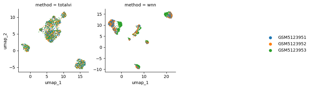
This unbalanced batch effect is also having an effect on WNN, but not on totalvi:

and the lisi scores confirm this view

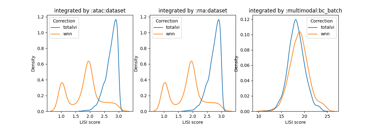
(the plot shows the same LISI score for atac:dataset and rna:dataset because the pipeline detects that the columns used for each integration performed are different)

Additionally, panpipes also computes scib-metrics to assess unimodal integration techniques with respect to batch correction and bio-conservation. Most of the metrics require cell type labels for each cell. For datasets where this information is not available at the time of integration, as is the case for the dataset in this tutorial, only few batch correction metrics can be calculated (no bio-conservation metrics) and plot generation is omitted. In any case, all computed metrics are saved as csv files for each modality separately. Let’s take a look at the metrics for the protein modality:

Embedding	ilisi_knn	pcr_comparison
Unintegrated	0.44926	0.0
bbknn	0.46967	0
harmony	0.89955	0.82495

Corroborating the previous findings, the harmony method seems to be the best choice for the protein modality in this dataset based on the scib batch correction metrics.

In the paper, we showcase how WNN offers the flexibility to integrate modalities that have individually been batch-corrected. To showcase this scenario, we will use the last functionality of panpipes integration workflow, the make merge_integration. This task should be run after you have inspected the results of the integration and have decided which of the applied corrections you want to keep, for both uni and multimodal approaches.

To do this, you must modify the pipeline.yml file and keep :

# -------------------------
# Creating the final object
# -------------------------
final_obj:
  rna:
    include: True
    bc_choice: scvi
  prot:
    include: True
    bc_choice: harmony
  atac:
    include: True
    bc_choice: bbknn
  multimodal:
    include: True
    bc_choice: WNN

and run

panpipes integration make merge_integration --local

once this is finished, you will find a new object in the main directory, namely teaseq_corrected.h5mu.

Let’s create a new directory inside the integration folder where we have just finished our run.

mkdir sub_integration && cd $_
ln -s ../teaseq_corrected.h5mu teaseq_temp.h5mu
cp ../pipeline.yml .

In the new pipeline.yml we have just copied over, modify the name of the input file to teaseq_temp.h5mu. Then set false all the modalities batch_correction algorithms, keep only wnn as a multimodal integration method and change the wnn parameters in the yaml file to instruct wnn to run on the batch corrected data from the prot and atac modalities in the h5mu input object, like so:

WNN:
    modalities: rna,prot,atac 
    batch_corrected:
      rna: scVI
      prot: harmony
      atac: bbknn

To compare the new vs the nobatch wnn run as we have done in integration, we can create a batch_correction directory in this subfolder and link the original file to this location by taking care of adding a string that will distinguish the original wnn run from this new one.

For example:

mkdir batch_correction && cd $_
ln -s ../../batch_correction/umap_multimodal_wnn.csv umap_multimodal_wnnnobatch.csv

Also, to avoid re-running the unimodal no_correction runs, we can link the individual modalities batch_correction/umap_*_none.csv in the same way.

Now go back to sub_integration directory and run again panpipes integration make full --local

The pipeline will pick the new requirement for wnn and create a new wnn run with the desired batch corrections for each modality, and since we have linked the previous wnn correction in this subdirectory, it will generate the outputs (check the figures folder for plots and scores) to compare wnn with and without batch correction.

When the run finishes, let’s inspect the new wnn run. As expected, the batch effect introduced by the prot modality is now accounted for.

To create a new mudata with this new version of wnn as well as the other corrections, we can link the unimodal correction files we generated before in the tmp folder:

cd tmp
ln -s ../../tmp/scvi_scaled_adata_rna.h5ad .
ln -s ../../tmp/harmony_scaled_adata_prot.h5ad .
ln -s ../../tmp/bbknn_scaled_adata_atac.h5ad .

We don’t need to change the pipeline.yml final bit because we are now fetching the updated wnn and the same unimodal correction methods as before. Run panpipes integration make merge_integration --local. The new teaseq_corrected.h5mu object now has the new wnn data in!