Ingesting multimodal (CITE-Seq + VDJ) datasets from cellranger outputs

Datasets and directories

Panpipes can read files from different cellranger outputs. Here we will showcase the example of two multmodal (CITE-Seq + VDJ) datasets from the 10x website while ingesting cellranger multi outputs.

Download dataset 1 ( 10k human PBMCs) from the 10x website

Download dataset 2 (CMV + 5K human Tcells ) from the 10x website

For this tutorial we downloaded the dataset 1 and dataset 2 files from the website and created folders within the ‘outs’ folder to simulate the directory structure of cellranger multi outputs as required by panpipes, as mentioned in our documentation on sample submission

# Here we show the directory structure of the outs folder for the 5k human CMV + Tcells dataset
# only with the essential files needed by panpipes ingest
tree -L 4 ./outs
outs
|-- multi
|   |-- count
|   |   |-- feature_reference.csv
|   |   |-- raw_feature_bc_matrix
|   |   |   |-- barcodes.tsv.gz
|   |   |   |-- features.tsv.gz
|   |   |   `-- matrix.mtx.gz
|   |   |-- raw_feature_bc_matrix.h5
|   `-- vdj_t
`-- per_sample_outs
    `-- human_cmv
        |-- count
        |   |-- feature_reference.csv
        |   |-- sample_filtered_barcodes.csv
        |   |-- sample_filtered_feature_bc_matrix
        |   |-- sample_filtered_feature_bc_matrix.h5
        |-- metrics_summary.csv
        `-- vdj_t
            |-- filtered_contig_annotations.csv

Submission and yaml file

We created a sample submission file which will instruct panpipes on how to find each modality’s path. Download this submission file here.

Besides the first column, “sample_id”, the order in which the columns are provided is not fixed, but the column names are fixed! Failing to specify the column names will result in omission of the modality from the analysis and early stopping of the pipeline.

We find useful to generate the submission file with softwares like Numbers or Excel and save the output as a txt file to ensure that the file is properly formatted. For more examples please check our documentation on sample submission files.

As we are ingesting CITE-Seq data, we created a protein metadata table, with information on if the antibody was an isotype or a hashing antibody. It is important to note that the first column is equivalent to the first column of cellranger’s features.tsv.gz. Download the protein metadata table for this tutorial here.

Run panpipes ingest

Now, activate the environment in which you have installed panpipes, create a 1_ingest folder and configure the ingest workflow within that folder

mkdir 1_ingest
cd 1_ingest
panpipes ingest config

panpipes ingest config This command will generate a config file, pipeline.yml. Modify the config file, or just use sample submission file we provided. You can find the preconfigured pipeline.yml file here.

As you see, since we have raw cellranger multimodal inputs, we can turn on a few tasks that require raw data, for example:

• parsing and plotting 10x metrics for all the modalities

plot_10X_metrics: True

• estimation of background signal for proteins and rna

assess_background: True

• normalization of the protein data using dsb

normalisation_methods: clr,dsb

Please remember to apply the necessary changes in this file to ensure it will run on your computer, and specify:

• the environment in which you’re running panpipes, if applicable.

• the path to the custom_genes_file that we use to run scanpy.score.genes (we provide an example file in the panpipes’ resources folder)

Now, run the full panpipes ingestion workflow with:

panpipes ingest make full

The pipeline will write to standard output and to a pipeline.log file about the steps it’s running. When it’s finished, you will see a pipeline finished message:

2023-11-27 10:07:10,498 INFO main task - Completed Task = 'pipeline_ingest.full' 
2023-11-27 10:07:10,499 INFO main experiment - job finished in 978 seconds at Mon Nov 27 10:07:10 2023 -- 27.26 12.18  0.14  0.52 -- 85d537bd-19b2-41cd-8134-5d615c1342e5

Panpipes ingest outputs

Let’s inspect the outputs we have generated with panpipes ingest in the ‘1_ingest’ directory”

tree -L 2 ./1_ingest
.
|-- 10x_metrics.csv
|-- _downsampled_cell_metadata.tsv
|-- figures
|   |-- atac
|   |-- background
|   |-- barplot_cellcounts_thresholds_filter.png
|   |-- prot
|   |-- rep
|   |-- rna
|   |-- rna_v_prot
|   `-- tenx_metrics
|-- logs
|   |-- assess_background.log
|   |-- concat_bg_mudatas.log
|   |-- concat_filtered_mudatas.log
|   |-- human_cmv_bg_downsampled.log
|   |-- human_pbmc_bg_downsampled.log
|   |-- load_bg_mudatas_human_cmv.log
|   |-- load_bg_mudatas_human_pbmc.log
|   |-- load_mudatas_human_cmv.log
|   |-- load_mudatas_human_pbmc.log
|   |-- plot_qc.log
|   |-- run_dsb_clr.log
|   |-- run_scanpy_qc_prot.log
|   |-- run_scanpy_qc_rep.log
|   |-- run_scanpy_qc_rna.log
|   |-- run_scrublet_human_cmv.log
|   |-- run_scrublet_human_pbmc.log
|   `-- tenx_metrics_multi_aggregate.log
|-- mm_bg.h5mu
|-- mm_cell_metadata.tsv
|-- mm_prot_qc_metrics_per_sample_id.csv
|-- mm_threshold_filter.tsv
|-- mm_threshold_filter_explained.tsv
|-- mm_unfilt.h5mu
|-- pipeline.log
|-- pipeline.yml
|-- scrublet
|   |-- human_cmv_doubletScore_histogram.png
|   |-- human_cmv_scrublet_scores.txt
|   |-- human_pbmc_doubletScore_histogram.png
|   `-- human_pbmc_scrublet_scores.txt
`-- tmp
    |-- human_cmv.h5mu
    |-- human_cmv_raw.h5mu
    |-- human_pbmc.h5mu
    `-- human_pbmc_raw.h5mu

The final MuData object with computed QC metrics is mm_unfilt.h5mu. A MuData object without QC metrics for each supplied sample in the sample submisison_file is also available and stored in the tmp folder (you can delete this folder to save space). The metadata of the final Mudata object is additionally extracted and saved as a tsv file, mm_cell_metadata.tsv. Lastly, the per sample ADT metrics for each antibody are extracted and also saved as a tsv file, mm_prot_qc_metrics_per_sample_id.csv.

Moreover a MuData object containing information for the background or the raw cellranger output is also created and is mm_bg.h5mu. This is either all the barcodes in the raw cellranger or a downsample object if the downsample param has been set to True in the pipeline.yml (in this case, we have set it to True).

The ingest pipleine also aggregates and outputs all the cellranger summary metrics for all the samples as a tsv file, 10x_metrics.csv.

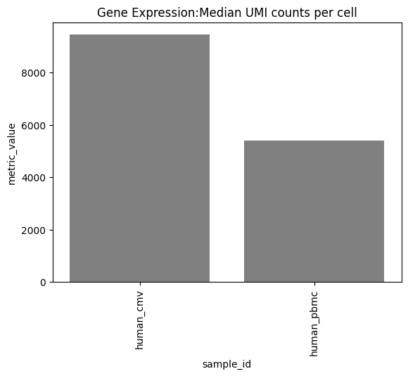
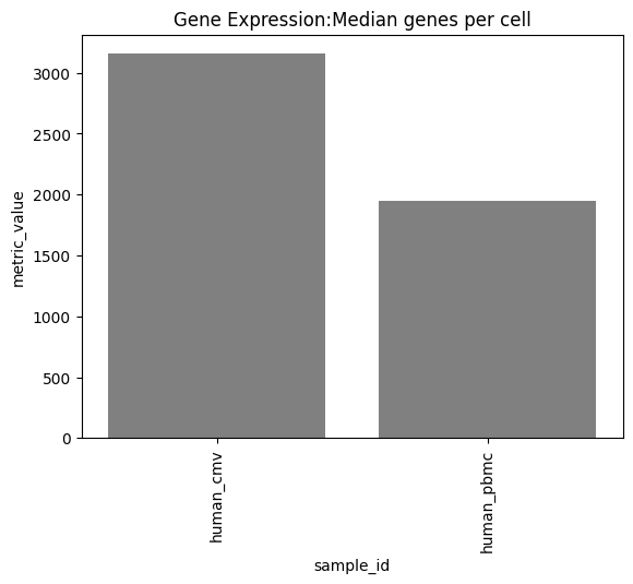
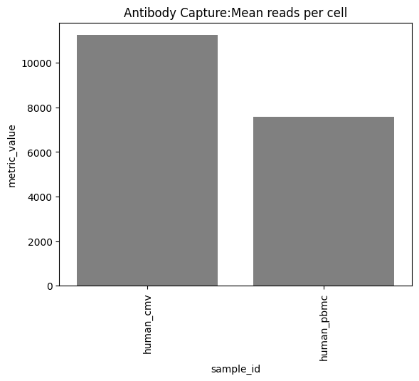
Additionaly, plots for all modalities for all the summary metrics are individually plotted across all samples and can be found under the figures/tenx_metrics directory. This is a nice way to compare and contrast all the samples in a single panpipes run for the relevant metrics.

10x metrics plots

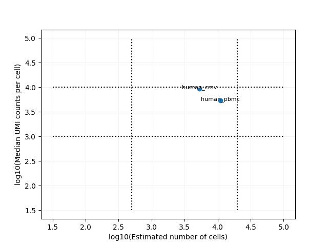
With the plots in the figures/tenx_metrics, you can evaluate the result of the cellranger multi run for your samples. For example, one can check the sequencing quality of the samples by evaluating:

1. the scatter plots of the number of cells vs the median umis in the log10 scale for the RNA modality.

2. the sequencing saturation per vs Number of reads per sample for the RNA modality.

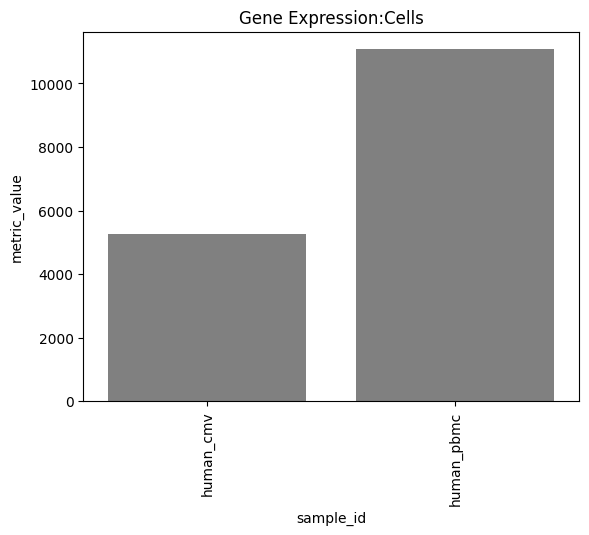
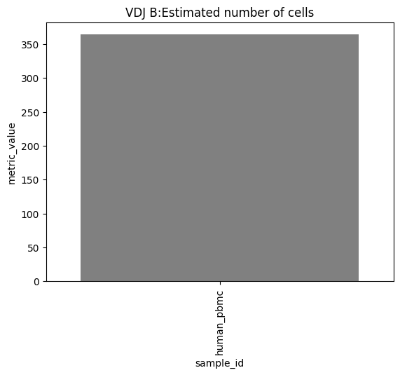
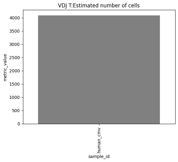
We also plots different metrics across all samples for all the inputted modalities. It might be useful to examine the number of cells across all the samples for rna + prot,BCR and TCR modalities.

one can also look at other relevant 10x_metrics such as the Mean or median reads/UMI counts/genes per cell for the different modalities.

Background plots

The ingest pipeline also plots the cumulative barcode rank plots for all samples (also known as “kneeplot”) , so that it is easier to contrast and compare them and evaluate the number of barcodes called as cells vs not. These plots can be found in figures/background

Moreover, we also evaluate the downsampled background for the rna and prot modality separately and compared to each for all samples. For example a scatter plot visualising the nUMI counts in the empty barcodes (background) vs the cell containing barcodes (foreground) in the protein vs rna.

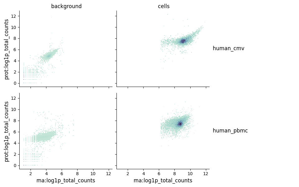
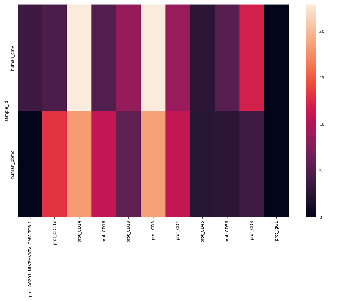
Additionally, we also plot the most highly expressed genes and proteins in the background as boxplots and heatmaps. This helps you evaluate potential sources of ambient contamination in the samples, like heamoglobin contamination or high mitochondrial gene expression or high background expression of particular antibodies.

RNA QC plots

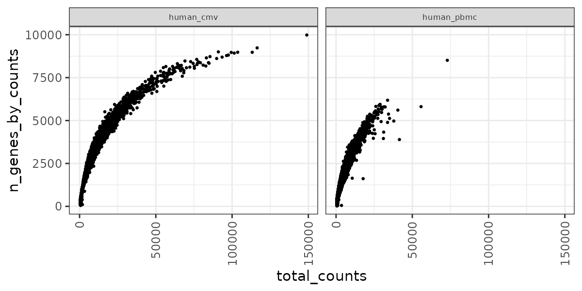
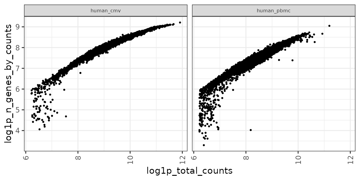
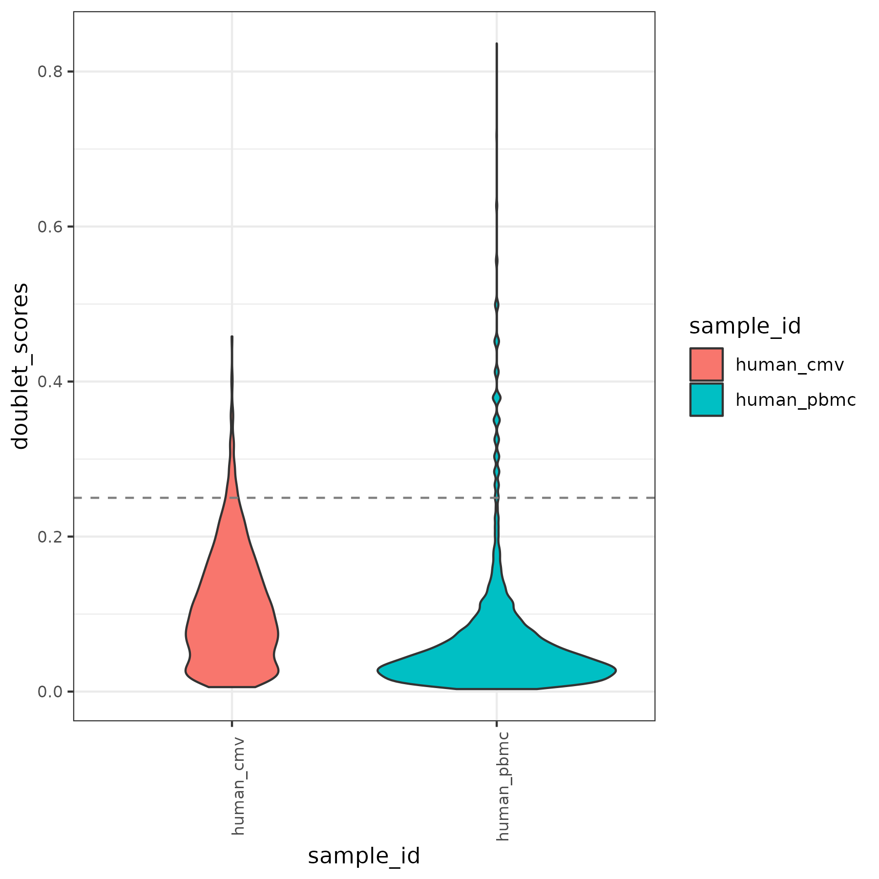
panpipes ingest workflow computes qc metrics for each modality given as input. For a multimodal sample it may be useful to check RNA metrics under the figures/rna such as number of genes detected in cells vs the total UMI counts , percentage of mitochondrial reads per cell vs library size and doublet scores across the different samples.

Protein QC and normalisation plots

For the PROT metrics it might be useful to check the total counts and mean counts of per ADT across samples. The figures can be found under figures/prot.

As for the prot modality clr and dsb normalisation can also be performed in the panpipes ingest step, we can also visualise the normalised ridge plots for 1) clr & 2) dsb normalisation for each of the ADTs for each sample in the sample_submission file.

The dsb normalisation corrects for background ADT noise and cell-to-cell technical variations and can help to identify a cleaner expression protein signal in comparison to the clr normalisation. Here we show the clr and dsb ridge plots for the human_cmv dataset.

Repertoire QC plots

For the QC of of VDJ data, we utilise the scirpy python package function scirpy.tl.chain_qc to perform QC based on the receptor-chain pairing configuration and categorise the cells into their receptor types and subtypes. This classification of the cells can be checked in the plots under figures/rep.

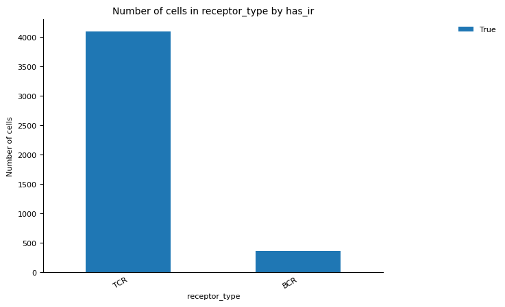
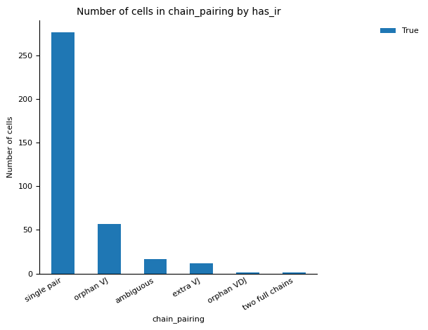
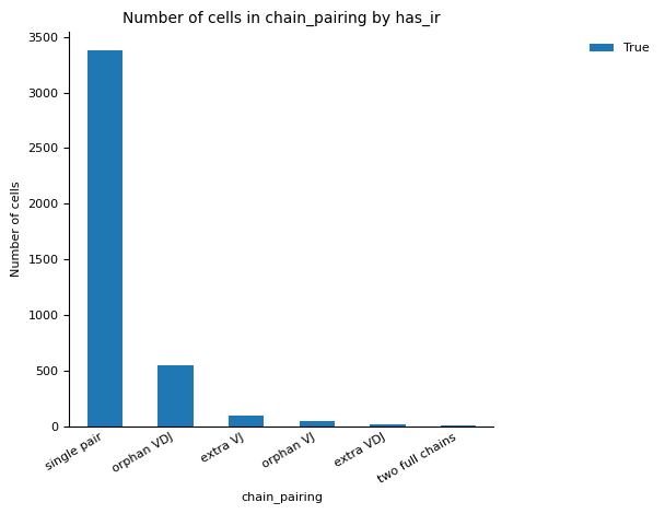
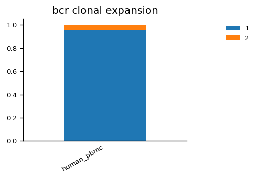
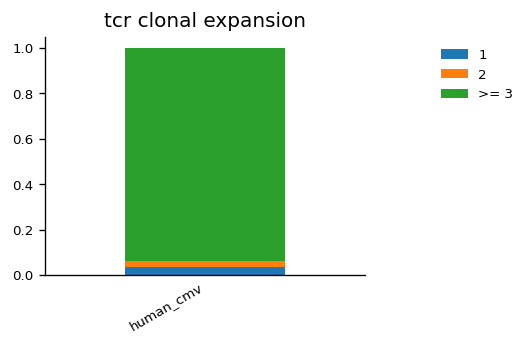
We can also visualise the proportion of cells belonging to expanded clonotypes for the TCR and BCR data across samples. For example in the human_cmv sample, we see there is a high fraction of cells with expanded TCR clones, but this is not the case of the BCR clones in the human_pbmc sample.

Multiple Filter threshold plots

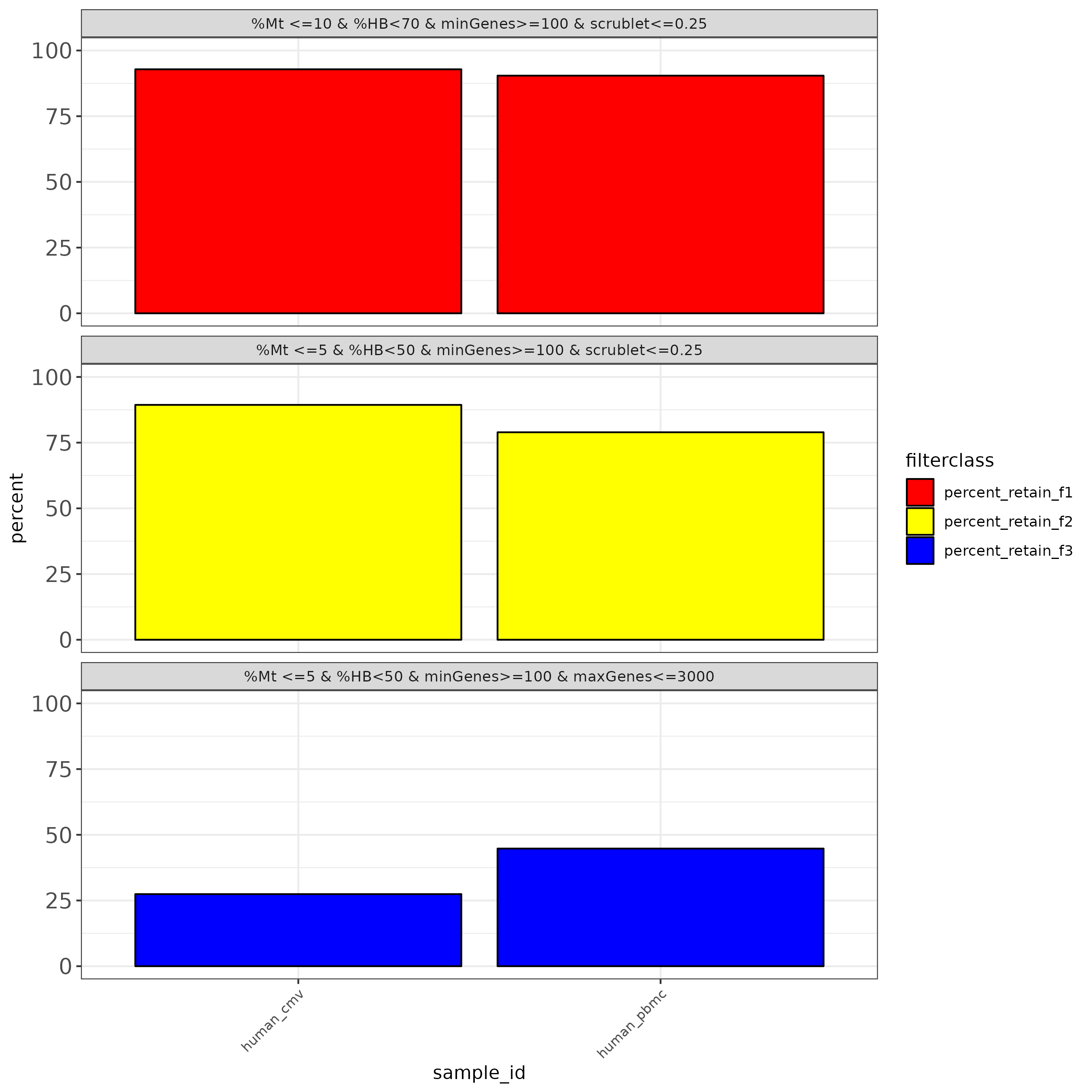
To aid with the filtering of the data, we also produce outputs that simulate common filtering scenarios, the height of the bar shows the percentage of cells retained if the threshold is applied.

Users can also inspect the unfiltered mudata generated file by reading it in a python session:

import muon as mu
mu.read("mm_unfilt.h5mu")

We have demonstrated how to run the ingest workflow on multimodal (CITE-Seq + VDJ) data with multiple samples. Filtering of cells and genes is not applied in the ingest workflow but in the preprocess. Inspecting these output should help the user to choose appropriate filters for their data!

Users can follow the preprocessing tutorial for an example on how to filter and further process the data.